EDA

Import control of corruption data

corruption = read_csv('.\\data\\corruption_EDA.csv')

Data Trend

corruption|> 
  group_by(year)|>
  summarise(mean = mean(signif(con_cor,4),na.rm = TRUE))|>
  ggplot(aes(x=year, y=mean)) +
  geom_point(color = 'red')+geom_line(aes(group=1),color = 'orange')+
  geom_smooth(se = FALSE,color = "purple")+
  labs(
    title = " Trend of control of corruption",
    x = "Year",
    y = "Control of corruption"
  )

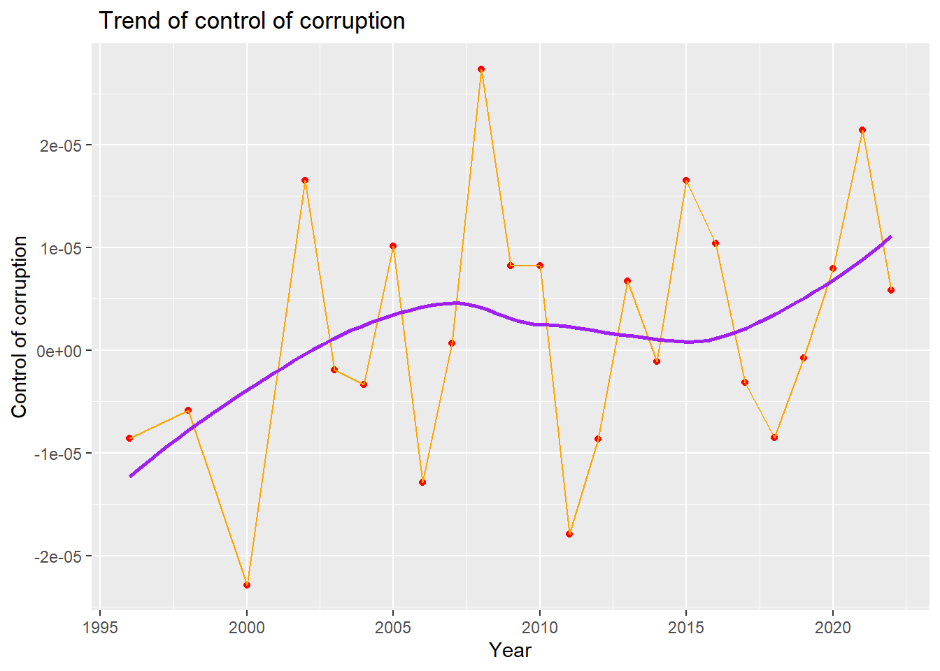
We draw a line plot with a smooth line to show the overall trend of control of corruption from 1996 to 2022. We can see from the plot, that there is a increasing trend for the control of corruption index from 1996 to 2007,and then declining trend from 2007 to 2015. From 2015 to 2022, there is a increasing trend for the control of corruption. In general, there is a increasing trend for control of corruption from 1996 to 2022.

With Governance Indicators

corruption %>% 
  select(con_cor,gov_eff,pol_vio,regu_qual,rul_law,voi_acc
) %>% 
  ggpairs(
    title = "Correlations Between govenance indicators",
    ggplot2::aes(alpha = 0.1)
  ) + 
  scale_fill_discrete() + 
  theme(axis.text.x = element_text(angle = 90, vjust = 0.5, hjust=1))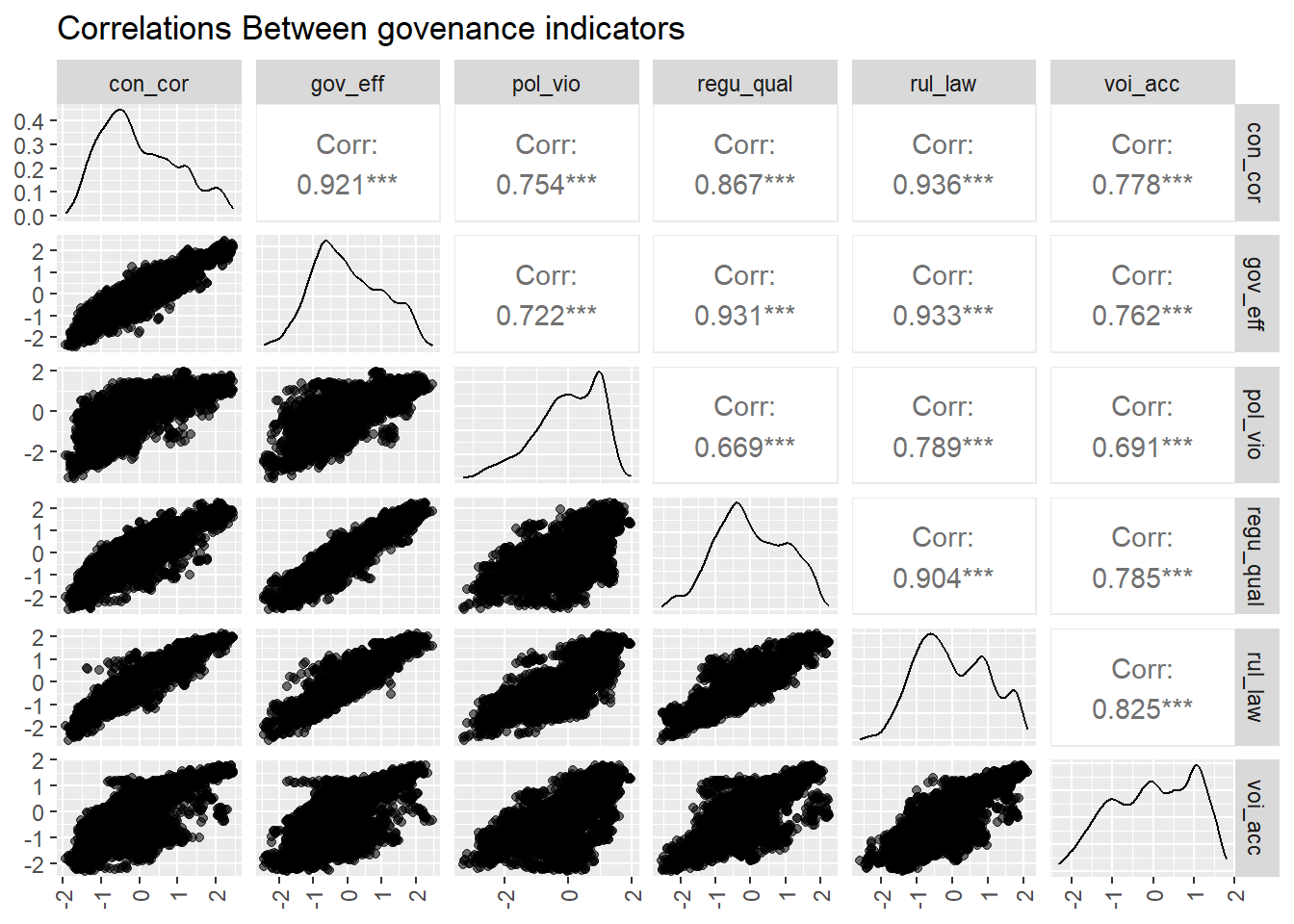

We also managed to show how control of corruption relate to other 5 types of governance indicator. The plot shows that the control of corruption has most significant correlation(bigger than 0.90) with government effectiveness and rule of law.

Then we make scatter plots of control of corruption and fit it with linear line against each of 5 types of governance indicators to visualize the relationship.

Level - 1

myplots <- vector('list', 4)
for (i in 2019:2022){
    myplots[[i-2018]] =
      corruption %>% 
      filter(year == i) %>% 
      ggplot(aes(x = gov_eff, y = con_cor))+geom_point()+geom_smooth(method = 'lm', se = TRUE, color = 'red')+labs(title = sprintf("year %s", i))

plot_row1 <- plot_grid(myplots[[1]], myplots[[2]])
plot_row2 <- plot_grid(myplots[[3]], myplots[[4]])
}
# title
title <- ggdraw() + 
  draw_label(
    "Control of corruption against effectiveness",
    fontface = 'bold',
    x = 0,
    hjust = 0
  ) +
  theme(
    # add margin on the left of the drawing canvas,
    # so title is aligned with left edge of first plot
    plot.margin = margin(0, 0, 0, 7)
  )
plot_grid(title,plot_row1,plot_row2 ,ncol=1,  label_size = 12,rel_heights=c(0.1, 1,1))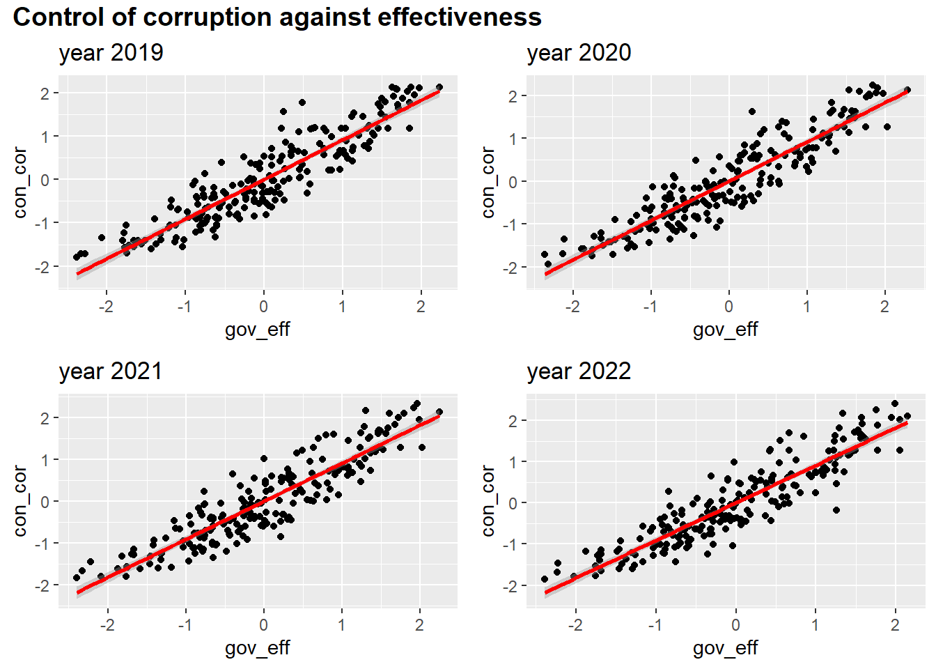

Level - 2

myplots <- vector('list', 4)
for (i in 2019:2022){
    myplots[[i-2018]] =
      corruption %>% 
      filter(year == i) %>% 
      ggplot(aes(x = pol_vio, y = con_cor))+geom_point()+geom_smooth(method = 'lm', se = TRUE, color = 'red')+labs(title = sprintf("year %s", i))
}

plot_row1 <- plot_grid(myplots[[1]], myplots[[2]])
plot_row2 <- plot_grid(myplots[[3]], myplots[[4]])
# title
title <- ggdraw() + 
  draw_label(
    "Con_cor against political stability and absence of violence terrorism",
    fontface = 'bold',
    x = 0,
    hjust = 0
  ) +
  theme(
    # add margin on the left of the drawing canvas,
    # so title is aligned with left edge of first plot
    plot.margin = margin(0, 0, 0, 7)
  )
plot_grid(title,plot_row1,plot_row2 ,ncol=1,  label_size = 12,rel_heights=c(0.1, 1,1))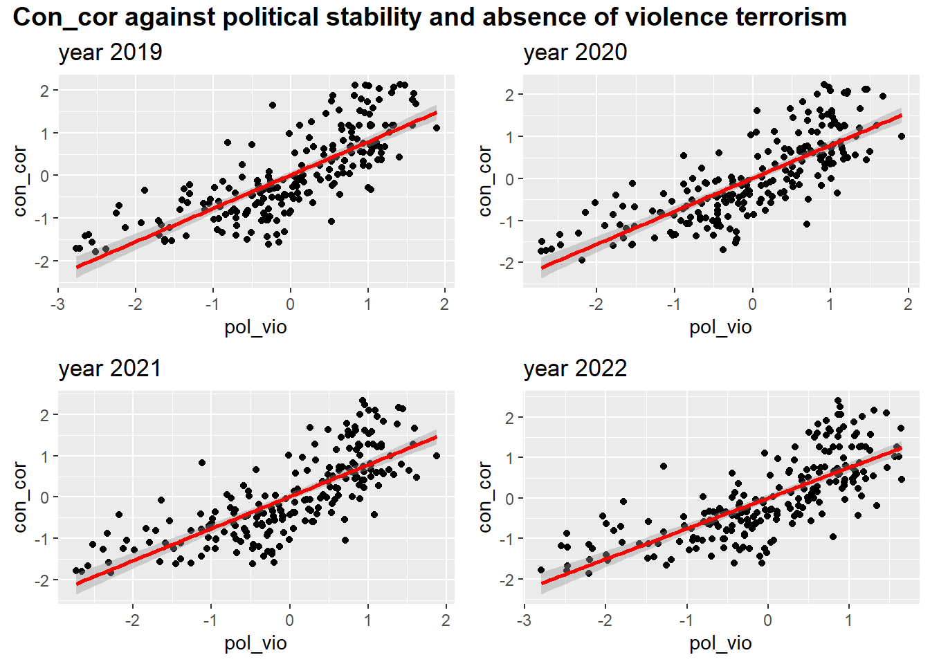

Level - 3

myplots <- vector('list', 4)
for (i in 2019:2022){
    myplots[[i-2018]] =
      corruption %>% 
      filter(year == i) %>% 
      ggplot(aes(x = regu_qual, y = con_cor))+geom_point()+geom_smooth(method = 'lm', se = TRUE, color = 'red')+labs(title = sprintf("year %s", i))
}

plot_row1 <- plot_grid(myplots[[1]], myplots[[2]])
plot_row2 <- plot_grid(myplots[[3]], myplots[[4]])
# title
title <- ggdraw() + 
  draw_label(
    "Control of corruption against regulatory_quality",
    fontface = 'bold',
    x = 0,
    hjust = 0
  ) +
  theme(
    # add margin on the left of the drawing canvas,
    # so title is aligned with left edge of first plot
    plot.margin = margin(0, 0, 0, 7)
  )
plot_grid(title,plot_row1,plot_row2 ,ncol=1,  label_size = 12,rel_heights=c(0.1, 1,1))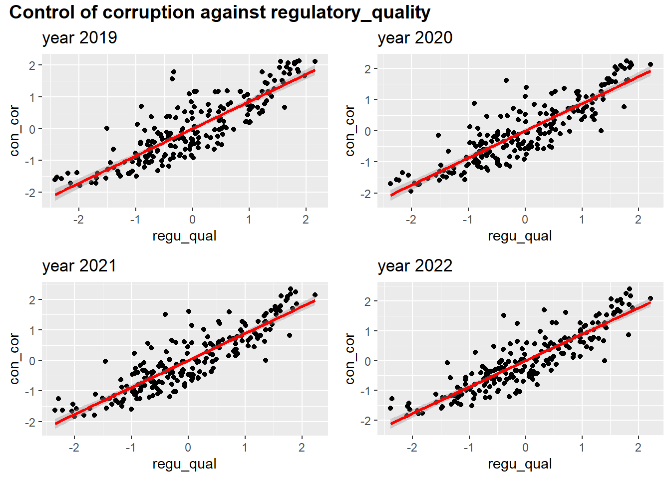

Level - 4

myplots <- vector('list', 4)
for (i in 2019:2022){
    myplots[[i-2018]] =
      corruption %>% 
      filter(year == i) %>% 
      ggplot(aes(x = rul_law
, y = con_cor))+geom_point()+geom_smooth(method = 'lm', se = TRUE, color = 'red')+labs(title = sprintf("year %s", i))
}

plot_row1 <- plot_grid(myplots[[1]], myplots[[2]])
plot_row2 <- plot_grid(myplots[[3]], myplots[[4]])
# title
title <- ggdraw() + 
  draw_label(
    "Control of corruption against rule of law",
    fontface = 'bold',
    x = 0,
    hjust = 0
  ) +
  theme(
    # add margin on the left of the drawing canvas,
    # so title is aligned with left edge of first plot
    plot.margin = margin(0, 0, 0, 7)
  )
plot_grid(title,plot_row1,plot_row2 ,ncol=1,  label_size = 12,rel_heights=c(0.1, 1,1))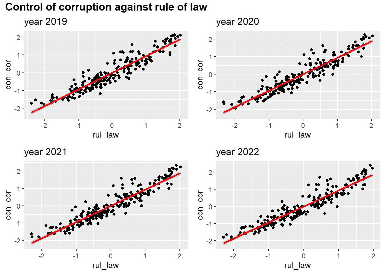

Level - 5

myplots <- vector('list', 4)
for (i in 2019:2022){
    myplots[[i-2018]] =
      corruption %>% 
      filter(year == i) %>% 
      ggplot(aes(x = voi_acc
, y = con_cor))+geom_point()+geom_smooth(method = 'lm', se = TRUE, color = 'red')+labs(title = sprintf("year %s", i))
}

plot_row1 <- plot_grid(myplots[[1]], myplots[[2]])
plot_row2 <- plot_grid(myplots[[3]], myplots[[4]])
# title
title <- ggdraw() + 
  draw_label(
    "control of corruption against voice and accountability",
    fontface = 'bold',
    x = 0,
    hjust = 0
  ) +
  theme(
    # add margin on the left of the drawing canvas,
    # so title is aligned with left edge of first plot
    plot.margin = margin(0, 0, 0, 7)
  )
plot_grid(title,plot_row1,plot_row2 ,ncol=1,  label_size = 12,rel_heights=c(0.1, 1,1))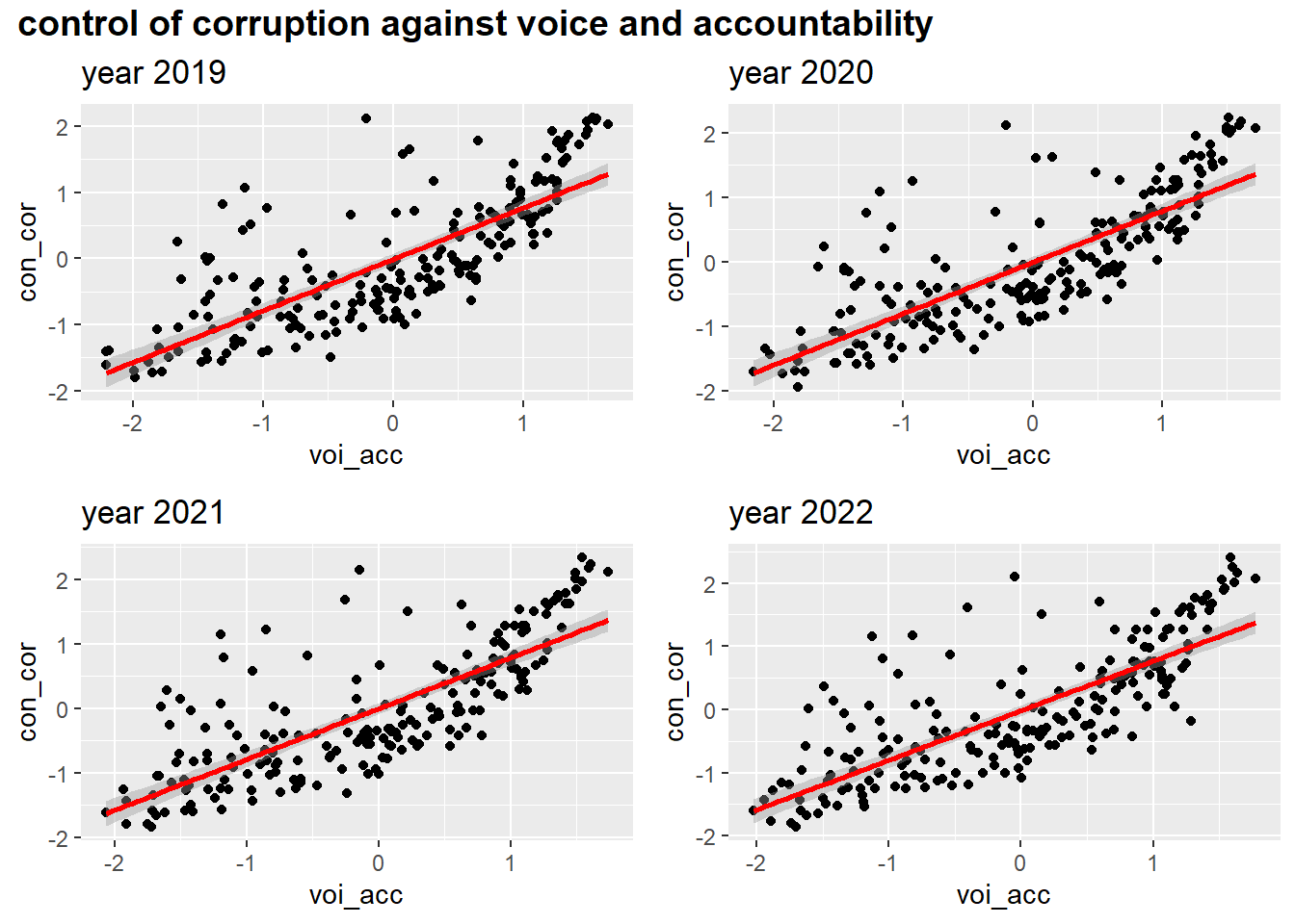

With Corruption by Development

Scatter Plot

corruption|>
  group_by(year,development)|>
  summarize(mean_cpi = mean(signif(con_cor,4),na.rm = TRUE))|>
  ggplot(aes(x = year,y = mean_cpi, group = development,color = development)) +
  geom_point(shape=19,size = 3)+geom_line()+
  labs(
    title = "Control of corruption over years by development",
    x = "Year",
    y = "Control of corruption")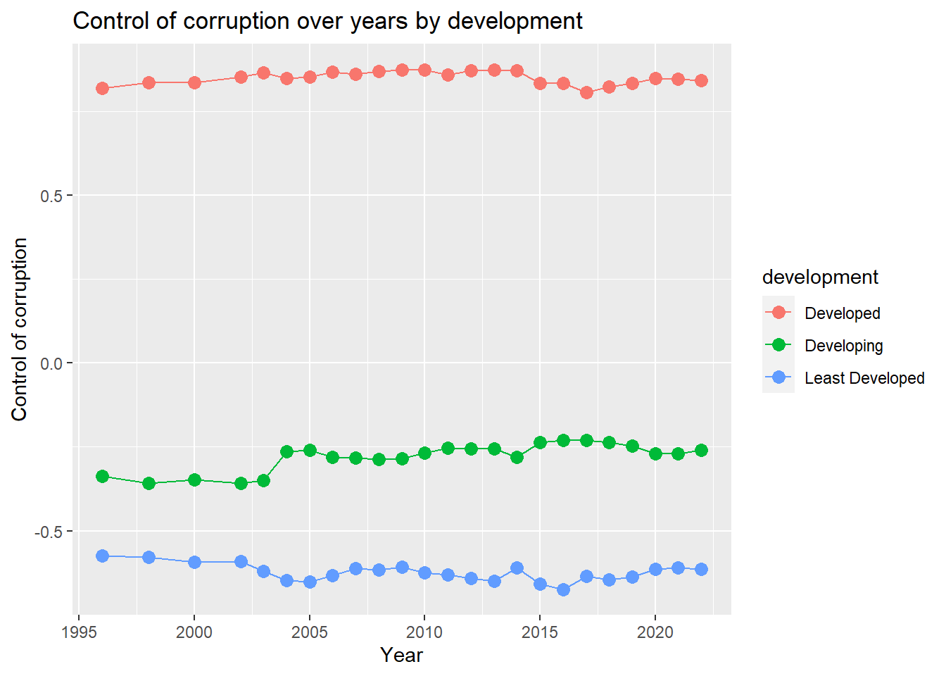

From the plot,We can see that the control of corruption for developing countries is getting better from 1996 to 2022 in general.For least developed countries, the control of corruption rate drops from 2002 to 2005 and then keeps fluctuation.For developed countries, the control of corruption index goes up from 1996 to 2014, and then falls.

Pie Plot

development_prop = corruption|>
  group_by(development)|>
  summarize(count = n_distinct(country_name))


myPalette <- brewer.pal(3, "Set2")
pie(pull(development_prop,count) , labels = c("Developed","Developing","Least Developed"), border="white", col=myPalette )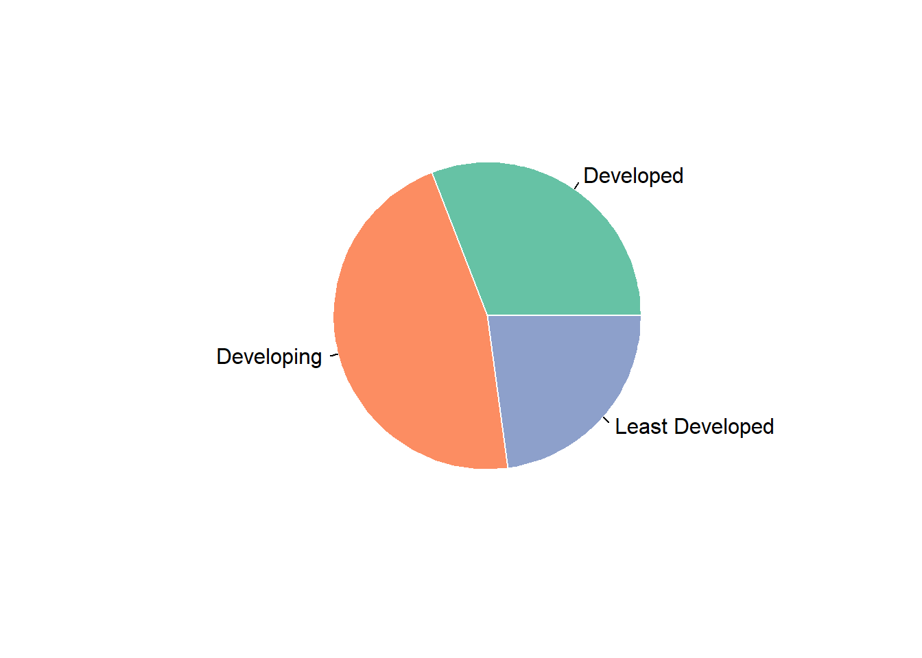

We have a pie plot for proportion of population by development.From the pie plot, we can read that developing countries account for the largest proportion. Developed countries is the second, and least developed countries is the third.

Together with the last plot, we can attribute the rising trend of control of corruption index over the world to rising trend of developing countries. The rising trend of developing countries outweigh the falling trend of least developed countries.

With Corruption by Continents

Continent is also a import factor we need to consider.We compares the population,gdp and control of corruption among continents by a series of plots.

mean_cpi = corruption|>
  group_by(continent)|>
  summarize(mean_cpi = mean(con_cor,na.rm=TRUE))|>
  ggplot(aes(x = continent,y = mean_cpi,fill = continent))+
  geom_bar(stat='identity')+
  labs(
    y = 'control of corruption'
  )

cpi_density = 
  corruption|>
  group_by(continent,country_name)|>
  summarize(con_cor = mean(con_cor,na.rm = TRUE))|>
  ggplot(
    aes(
      x = con_cor
    )
  ) + 
  geom_density(aes(fill = continent), alpha = 0.15) + 
  labs(
    x = "control of corruption",
    y = "Density"
  )
cpi_continent = mean_cpi/cpi_density
cpi_continent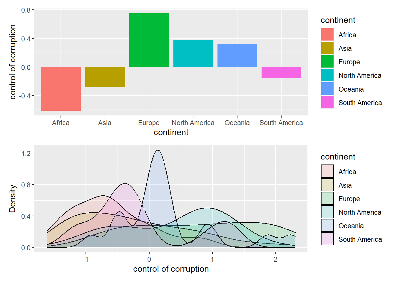

We draw a bar plot of mean control of corruption index by continents and a density plot to show the distribution of control of corruption index. From the histogram, we can see that Europe has the highest control of corruption index, whereas Africa has the lowest one.

With GDP

mean_gdp = corruption|>
  group_by(continent)|>
  summarize(gdp = mean(gdp,na.rm=TRUE))|>
  ggplot(aes(x = continent,y = gdp,fill = continent))+
  geom_bar(stat='identity')+
  labs(
    y = 'Mean GDP'
  )

gdp_density = corruption|>
  group_by(continent,country_name)|>
  summarize(gdp = mean(gdp,na.rm = TRUE))|>
  ggplot(
    aes(
      x = gdp
    )
  ) + 
  geom_histogram(aes(fill = continent), alpha = 0.5) + 
  labs(
    x = "GDP",
    y = "Density"
  )
gdp_continent = mean_gdp/gdp_density


gdp_continent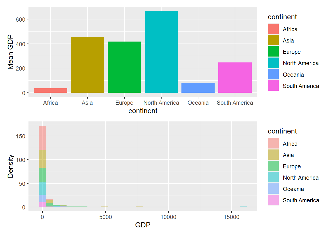

The upper bar plot shows mean GDP of countries in each continent.The lower histogram plot shows the distribution of GDP in each continent. We can get that North America has the highest mean GDP, and Africa has the lowest mean GDP.

With Population

Plot - 1

corruption %>%
  ggplot( aes(x=continent, y=population, fill=continent)) +
    geom_boxplot() +
    scale_fill_viridis(discrete = TRUE, alpha=0.6) +
    geom_jitter(color="red", size=0.4, alpha=0.9) +
    theme_ipsum() +
    theme(
      legend.position="none",
      plot.title = element_text(size=11)
    ) +
    ggtitle("Population among continents") +
    ylab("Population")+
    xlab("Continent")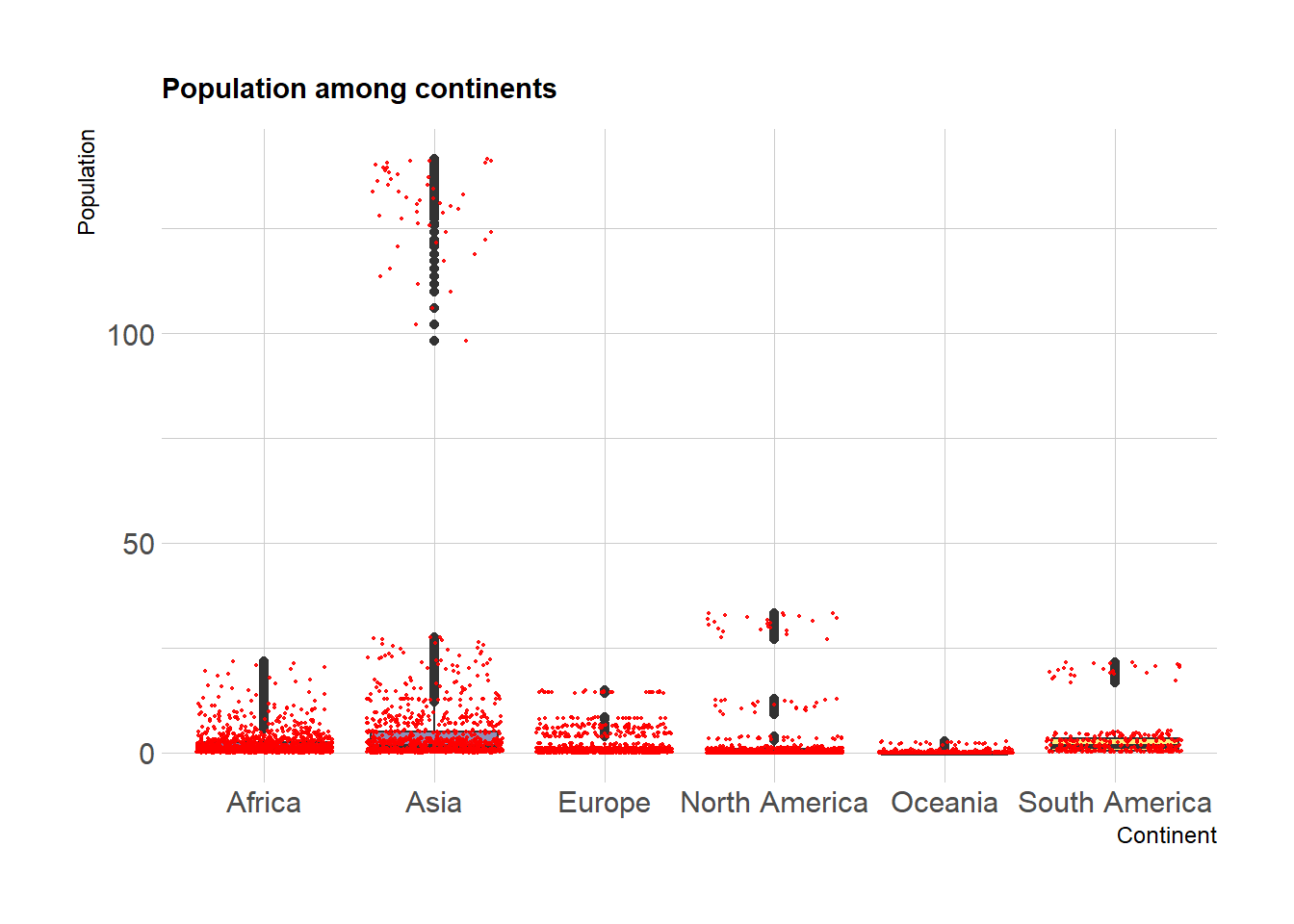

Based on the boxplot of population distribution among countries in each continent, we can read that Asia is the most populated area, and populated countries in North America has larger population than those countries in Europe. Oceania is the least populated area.

Plot - 2

myplots <- vector('list', 4)
for (i in 2019:2022){
    myplots[[i-2018]] =
      corruption %>% 
      filter(year == i) %>% 
      ggplot(aes(x = gdp_per_capita
, y = con_cor))+geom_point(color = 'purple')+geom_smooth(method = 'lm', se = FALSE, color = 'pink'
)+labs(title = sprintf("year %s", i))+ xlab("GDP per capita")
}

plot_row1 <- plot_grid(myplots[[1]], myplots[[2]])
plot_row2 <- plot_grid(myplots[[3]], myplots[[4]])
# title
title <- ggdraw() + 
  draw_label(
    "Corruption against GDP per capita",
    fontface = 'bold',
    x = 0,
    hjust = 0
  ) +
  theme(
    # add margin on the left of the drawing canvas,
    # so title is aligned with left edge of first plot
    plot.margin = margin(0, 0, 0, 7)
  )
plot_grid(title,plot_row1,plot_row2 ,ncol=1,  label_size = 12,rel_heights=c(0.1, 1,1))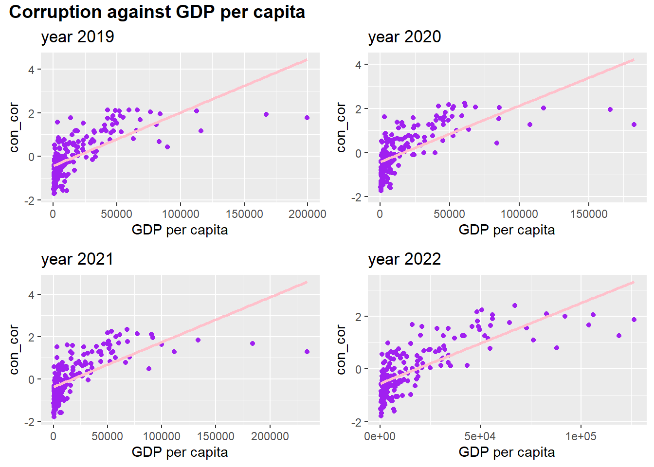

In addition, we also draw a scatter plot to check the relationship between control of corruption and GDP per capita.We can read that control of corruption is positively proportional to GDP per capita. However, when GDP per capita is high, the control of corruption keeps stable and does not follow the rising trend of GDP per capita.